Methods
Summary of the methods used to define indicators, analyze data, and present information for Tolko's Southern Operating Area.

Number of ABMI sites in Tolko's Southern Operating Area:
The ABMI monitors the state of Alberta’s land cover and biodiversity, including in the Southern Operating Area. Methods are summarized for:
- Land cover metrics, including: human footprint, vegetation cover, landbase change, native habitat, and linear feature density.
- Biodiversity metrics, including: Biodiversity Intactness Index, sector effects, and land base change attribution.
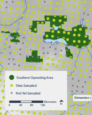
Location of ABMI monitoring sites within Tolko's Southern Operating Area.
Introduction
From the boreal forest in the north to the grasslands in the south, the ABMI monitors the state of Alberta’s biodiversity.
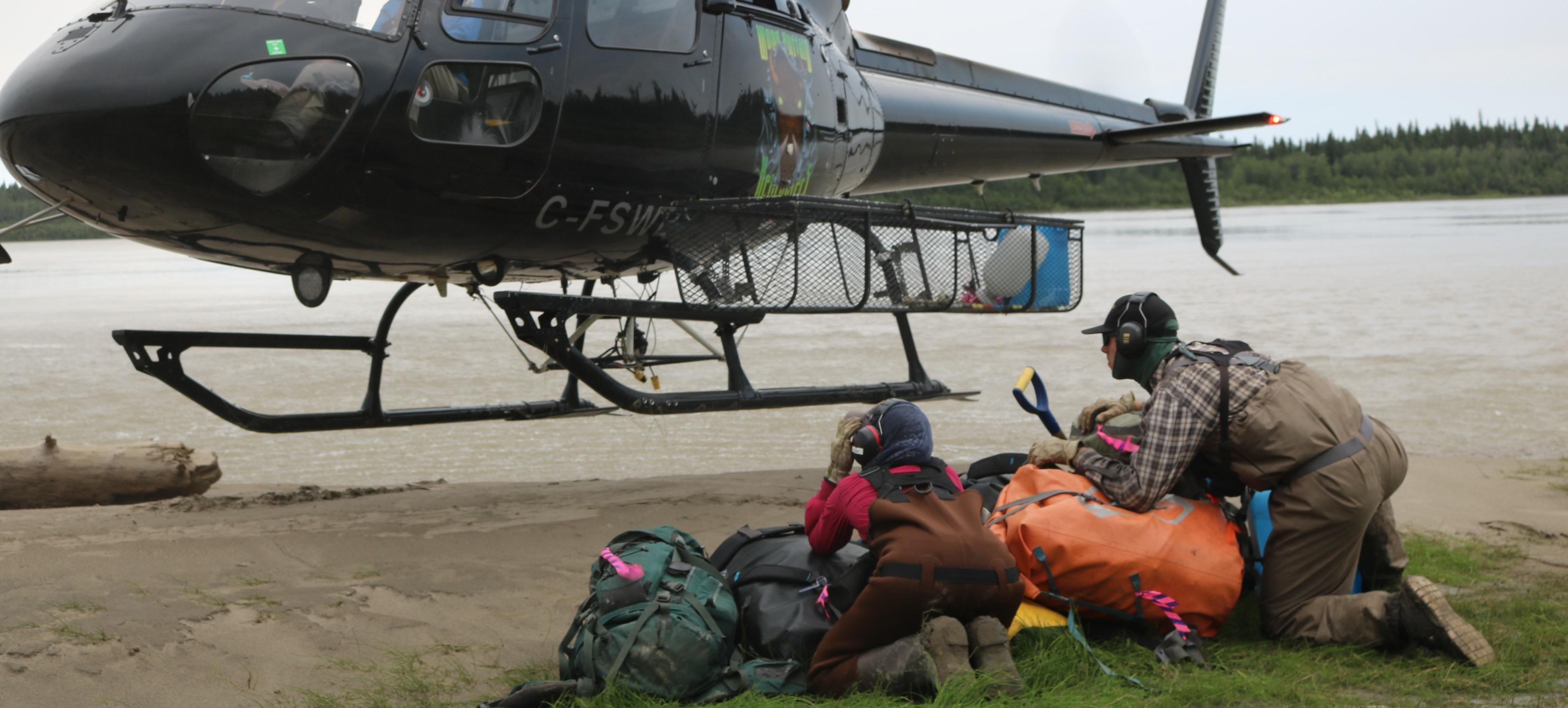
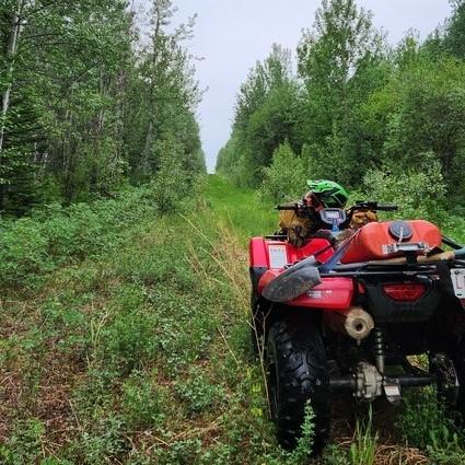
The ABMI employs a systematic grid of 1,656 site locations, spaced 20 km apart, to collect biodiversity information, including species and habitat data, at both terrestrial and wetland sites[1]. We also monitor at other “targeted” sites as needed to address additional monitoring and research objectives.
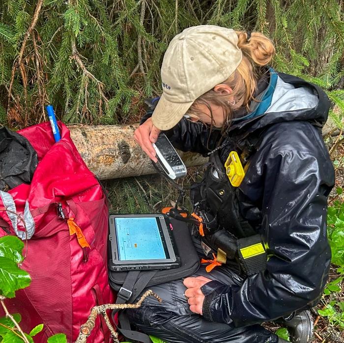
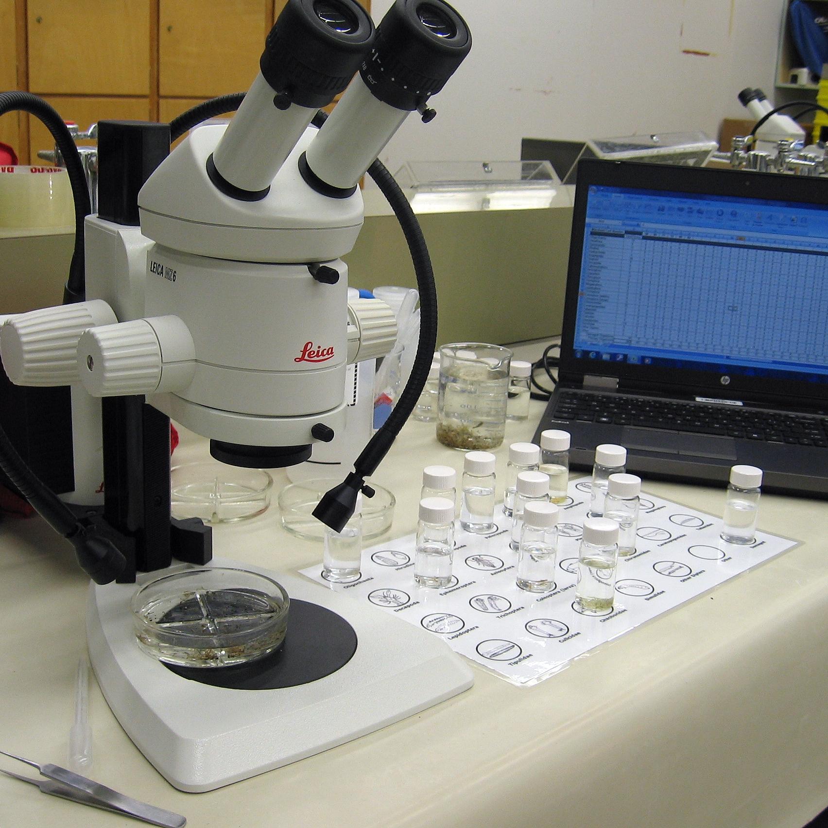
At each location, ABMI technicians record the species that are present and measure a variety of habitat characteristics. For species that cannot be identified in the field (e.g., soil mites and lichens), samples are sent to ABMI taxonomists to sort, identify, and archive to complete our species-level dataset.
Methods
Click on a tab for a summary of methods used to analyze land cover and biodiversity results for Tolko’s Southern Operating Area:
Human Footprint and Vegetation
Measuring Human Footprint
Definition of Human Footprint
The ABMI defines human footprint as the visible alteration or conversion of native ecosystems to temporary or permanent residential, recreational, agricultural, or industrial landscapes. The definition includes all areas under human use that have lost their natural cover for extended periods of time, such as cities, roads, agricultural fields, and surface mines. It also includes land that is periodically reset to earlier successional conditions by industrial activities such as forest harvest areas and seismic lines.
Some human land uses, such as grazing, hunting, and trapping, or the effects of pollution, are not yet accounted for in our human footprint analyses. The ABMI is continuously working to improve human footprint products, using the reference data and expertise of authorities within the Government of Alberta.
Human Footprint Categories
Human footprint is divided into eight categories for analysis:

Agriculture Footprint: Areas of annual or perennial cultivation, including crops and tame pasture, as well as confined feeding operations and other high-density livestock areas.

Energy Footprint: Areas where vegetation or soil has been disturbed by footprint types associated with the energy sector, including mine sites, pipelines, seismic lines, transmission lines, well sites, and wind-generation facilities. This category also includes industrial facilities related to the oil and gas sector, such as refineries, plants, compressor stations, and flare stacks.
Forestry Footprint: Areas in forested landscapes where timber resource extraction has occurred for industrial purposes, including clear-cut and partial-cut logging methods.

Forestry Footprint, Net: The area of forestry footprint prorated for how much it has recovered for biodiversity, based on harvest area age and stand type (deciduous or conifer). A newly harvested area is considered to be 0% recovered, while mature forest is 100% recovered. This is not to say that a recent harvest area has no biodiversity value, just that its biodiversity is as different from the original mature/old forest as it will ever be when it is first harvested.

Human-created Waterbodies: Human-created waterbodies created for a variety of purposes, such as to extract fill (borrow-pits, sumps), water livestock (dugouts), transport water (canals), meet municipal needs (water supply and sewage), and store water (reservoirs).

Transportation Footprint: Railways, roadways, and trails with hard surfaces such as cement, asphalt, or gravel, roads or trails without gravel or pavement, and the vegetation strips alongside transportation features.

Urban/Industrial Footprint: Residences, buildings, and disturbed vegetation and substrate associated with urban and rural settlements, such as housing, shopping centres, industrial areas, golf courses, and recreation areas, as well as bare ground cleared for industrial and commercial development. This category does not include industrial facilities associated with the oil and gas industry; these feature types are included in the Energy Footprint category.
Total Human Footprint: Summary of six human footprint categories combined: agriculture, energy, forestry, human-created waterbodies, transportation, and urban/industrial.
How Human Footprint is Analyzed and Reported
The ABMI monitors the status of Alberta’s human footprint using satellite imagery at two spatial scales:
Provincial Scale
At the provincial scale, the ABMI merges 20 human footprint sub-layers (based on 117 feature types) into a single integrated layer by applying a specific order of precedence to create the ABMI Human Footprint Inventory (HFI). Some of these 20 sub-layers are created by the ABMI and Government of Alberta as part of the Alberta Human Footprint Monitoring Program. We used the HFI for 2010 and 2021 conditions in this report.
We use the HFI from 2021 for three purposes in this report:
- to standardize the 3×7-km human footprint trend estimates before reporting,
- as part of the analysis of biodiversity intactness and sector effects to identify how the occurrence and relative abundance of species varies in relation to native land cover, human footprint, and spatial/climate variables, and
- to generate maps of human footprint in Tolko’s Southern Operating Area.
We use HFI 2010 as part of land base change analyses, reporting on change in several land cover indicators between 2010 and 2021.
This product is updated approximately every two years; the data and the metadata associated with this product are available here.
3 x 7-km Samples
The ABMI uses human footprint data measured annually at a 1:5,000 scale to track changes in human footprint over time. Detailed annual samples of human footprint are measured in a 3 × 7-km rectangular area centred near each of the ABMI’s 1,656 sites, which when summed across all sites amounts to about 5% of the province’s land surface. ABMI human footprint trend data are available for 1950, 1985, 2000, 2001, and 2004 to 2021. Trend data and the metadata associated with these data can be accessed here.
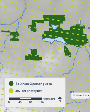
Distribution of ABMI 3x7-km detailed annual sampling sites in the Southern Operating Area.
Human Footprint Recovery
As a successional footprint, forestry recovers with time after disturbance. To account for this recovery, we summarize “recovered forestry”—defined as Forestry, Net in this report—prorating the effects on biodiversity of older harvested areas using biotic recovery curves based on a literature review of the recovery of forest species in harvest areas of different ages[2]. A newly harvested area is considered to be 0% recovered, while a mature/old forest is 100% recovered. Field studies of the abundance of species in harvest areas of different ages were used to fill in the recovery curve between those two benchmarks. Because results show faster recovery in deciduous forest than in conifer forest, we apply different recovery curves for these two forest types. More information on the curves used is available in the ABMI’s Status of Human Footprint in Alberta report. We do not yet have information on recovery of other types of human footprint.
Reporting on Human Footprint
To report on the status of human footprint (Section 2.1), the ABMI presents the percentage of land directly altered by human activities, ranging from 0% (no visible human footprint) to 100% (completely modified by human footprint). In general, cities and cultivated fields have high human footprint, while protected and undeveloped areas have low human footprint. We summarize total human footprint and the seven reporting categories.
Trend in human footprint in Tolko’s operating areas was assessed using the 3×7-km detailed inventory of human footprint available for: 1950, 1985, 2000, 2001, 2004–2021. Trend is presented for total human footprint and the seven reporting categories. The maps used to visualize human footprint in this report are based on the HFI 2021 (described above).
Measuring Vegetation
Backfill Vegetation Layer
The backfill vegetation layer or reference/native vegetation layer pre-human disturbance was created by the ABMI through the amalgamation of existing information on vegetation, habitat and soil throughout Alberta. To obtain a seamless reference vegetation layer, vegetation in human footprint was replaced by vegetation predicted to be present in the absence of human footprint (i.e., human footprint was "backfilled" to native vegetation). More information on this product can be found here.
Forested vegetation is classified into six categories: upland deciduous, mixedwood, pine, or spruce (including true firs), and lowland treed bogs, treed fens, and treed swamps. For all forested vegetation classes, except for treed fens and treed swamps, we assigned age classes of 0–9 years, 10–19 years, 20–39 years, continuing in 20-year classes through to the oldest class of 160+ years. Non-forested vegetation is classified into nine categories: upland grass and shrubs, shrubby fens, bogs and swamps, graminoid fens, marshes, open wetlands and bare areas.
The ABMI’s backfill vegetation layer combined with the ABMI human footprint is used to summarize the effects of land base change on different vegetation types, and as part of statistical modeling to determine cumulative effects of human footprint (Biodiversity Intactness, Sector Effects) and land base change (Attribution) on species habitat.
Vegetation Categories
Results for 10 vegetation types are summarized in this analysis:
- Upland forest types: deciduous, mixedwood, pine, White Spruce.
- Lowland forest types: Black Spruce, treed fen
- Other vegetation types: swamp (treed and non-treed), open wetland (shrubby and graminoid), and upland grass and shrub.
In addition, we summarized information for old forests (both upland and lowland) which we define as stands greater than 120 years old.
Reporting on Vegetation
To report on the status of vegetation (Section 2.2), the ABMI presents the percentage of each vegetation type directly after accounting for human footprint on the land base, ranging from 100% coverage of a vegetation type (no visible human footprint) to 0% (completely modified by human footprint).
Trend in vegetation types in Tolko’s operating areas was assessed by overlaying the 3×7-km detailed inventory of human footprint onto the backfilled vegetation layer and summarizing percent area of vegetation types left undisturbed. Results for trend in overall cover for the 10 vegetation types is available for: 1950, 1985, 2000, 2001, 2004–2021. Trend in old forest categories (>120 years) covers 2000–2021 because we are uncertain about how well we can “back-cast” forest ages to historical times.
Land Base Changes
Land Base Changes: 2010 to 2021
To summarize land base changes between 2010 and 2021, the 2010 and 2021 wall-to-wall vegetation and human footprint maps were intersected, and transitions of land base cover types were summarized. Six causes of change are distinguished:
- Aging of native forest that is undisturbed over that span,
- Aging of harvest areas that existed in the first year,
- Fires,
- New forestry footprint,
- New non-forestry human footprint replacing native habitat and harvest areas, and
- Changes in non-forestry human footprint that existed in the first year.
Currently only undisturbed forest stands and forestry footprint age in the land base summaries. Other human footprint continues to exist unchanged unless it is replaced by a different type of human footprint; as a result, component 6 is always small.
In this report, the following summaries are provided for the Southern Operating Area:
Disturbances in Broad Native Vegetation Types
Broad vegetation types (stand types combining all age classes, open vegetation types) can be affected by fire, new forestry footprint, and new non-forestry footprint. Aging of undisturbed vegetation does not need to be reported for these broad types—any stand that was not disturbed necessarily aged 11 years in the 2010 to 2021 time span. We do not “retire” human footprint, and back-filled vegetation types do not change, so there is no way that any area can be recruited into these broad vegetation types.
Figures in Section 2.3 show the areas of the three disturbance types and the area that remained undisturbed for each vegetation type. Results are presented as raw areas, and also as percentages of the 2010 area of each vegetation type.
Changes in Old Stands
Old stands can also be reduced by fire, new forestry human footprint, and new non-forestry human footprint. Unlike the ageless broad vegetation types above, old forest can also recruit as undisturbed stands cross the “old” age threshold. These processes are summarized for old stands (120+ years) in the four upland stand types (deciduous, mixedwood, pine, White Spruce).
Figures in Section 2.3 show the area of old forest of each stand type lost to the three disturbance processes and the area recruited due to aging of undisturbed stands. Results are also presented as a percentage of the 2010 area of each old forest type.
Land Base Changes due to 2023 Fires
We used the 2021 wall-to-wall vegetation+ human footprint map, then added fires from 2022 to form the “veg2022+HF2021” layer (generally called “2022 layer” below). This is the baseline to assess the effects of the 2023 fires against. Fire polygons from the 2023 fire season were downloaded on Oct. 15, 2023, when most of the season’s fires were out or not growing. These fires were overlaid on the veg2022+HF2021 baseline to produce the “veg2023+HF2021” layer (generally called “2023 layer” below). The comparison here is just the changes due to the 2023 fires, without any human footprint in 2023 (or in 2022), because those human footprint layers won’t be ready for some time. This means that a small proportion of the area that we report as native vegetation affected by fire would actually have been human footprint from 2022 or the first nine months of 2023.
The 2023 current fire map is approximate, as detailed mapping has not been completed on most large, complex fires, some of which were still active at the time of reporting. Fire skips within large fire areas have generally not been mapped yet.
Summaries of land base change due to the 2023 fires in the Southern Operating Area (Section 2.4) include area and percentage burned for: 1) Each broad vegetation type, 2) Old upland stand types, where “old” is defined as 80+ years or 120+ years, 3) Forestry harvest areas, grouped as deciduous versus conifer, or <20 years old versus 20+ years old. An additional summary calculated average stand age for different stand types before versus after the 2023 fires, with the fires resetting stand age to 0, and unburned stands aging one year over that time span.
Changes in Average Age of each Forest Type
Change in average stand age is a useful land base indicator because it shows whether disturbances are being balanced by aging of undisturbed stands. Change in average age from 2010 to 2021 was calculated for six stand types: deciduous, mixedwood, pine, White Spruce, treed lowlands (combined), and all stand types. We also partition out changes due to natural and harvested stands aging, fires, new forestry, and new non-forestry human footprint.
The areas of each age class were used to calculate (area-weighted) average age of each stand type in 2010, using the mid-range age of the age class (5 for 0–10, 30 for 20–40, etc), and 180 for age class 9 (=160+ year). Undisturbed native and harvested stands aged 11 years over the 11-year time span. Burned and harvested stands reverted to age 0 + 5.5 years (assuming they were harvested on average at the middle of the 11-year span). New non-forestry human footprint became age 0 and stayed at that age. Fire and footprint therefore cause a reduction in average age, with the extent of the reduction for a given area of land depending on how old the stand was prior to the disturbance. The 2021 average age is the 2010 average age plus these area-weighted positive contributions from aging and negative contributions from disturbance.
For each stand type, figures in Section 2.5 show the average age in 2010 and 2021, and the changes due to the aging and disturbance components.
Native Habitat
Native Habitat
Through mapping all human footprint in the province, the HFI allows areas of native terrestrial habitat to be identified—in other words, those areas in the province that have not been visibly disturbed by humans, although natural disturbances (e.g., wildfire, insect outbreaks) and invisible effects of humans (e.g., pollution) still occur. Further, the ABMI can track the amount of interior native habitat that is effectively “away” from the influence of human footprint due to edge effects. To report on the status of native vegetation, we present:
- The percentage area of land cover that has no visible human footprint (although land uses like grazing may still occur).
- The percentage area of interior native vegetation using three edge distances applied outwards from human footprint—50 m and 200 m following recommendations from Huggard and Kremsater (2015[3]), and 500 m to represent the longest reported or policy-based edge effects, such as those for Woodland Caribou. These three edge distances are called “base” distances. The base distances are narrowed to account for two factors (for detailed methods see Huggard and Kremsater 2015[2]).
- Width of human footprint. For narrow human footprint types like linear features, the edge influence that extends into native habitat is reduced because these openings have little surface wind, are shaded in most orientations, and are considered to be under “forest influence” for many species. As an exception, roads are assigned the full buffer distance regardless of road width, to conform to Government of Alberta methods for interior habitat.
- Recovery of forestry footprint. The edge distance is reduced as forestry footprint recovers (ages).
See Section 2.6 for native habitat results.
Linear Features
Linear Features
Linear features are analyzed using polylines (lines centered on the width of the line) of these feature types, and are summarized as density of linear footprint in km/km2. Some linear features, such as low-impact seismic lines, are not included. The ABMI is continuously working to improve linear footprint products, using the reference data and expertise of authorities with the Government of Alberta. Linear feature types are divided into the following categories for analysis:

Conventional Seismic Line: A seismic line that was constructed prior to the use of Low-Impact-Seismic (LIS) construction methods. Conventional seismic lines, also referred to as legacy seismic lines, were constructed using older technology that required the lines to be between 5 to 8 m in width to allow equipment to operate on the lines.
Pipeline: A line of underground and overground pipes, used for the delivery of fluids such as petrochemicals, as well as the physical clearing around the pipeline(s).
Road: Roadways paved with asphalt or concrete, roads surfaced with gravel and which serve as a main access route, as well as airplane runways and interchange ramps. Included are roads surfaced with dirt and/or low vegetation which serve as minor access routes.
Transmission Line: Utility corridor greater than 10 m wide with poles, towers, and lines for transmitting high-voltage (> 69 kV) electricity.
Railway: Corridors created for railways, as well as the physical clearing around the railway.
Total Linear Footprint: Summary of all linear footprint categories combined.
See Section 2.7 for linear features results.
Biodiversity Intactness
Biodiversity Intactness
Methods for calculating Biodiversity Intactness and sector effects are summarized below. For a detailed description of methods, see Sólymos et al. (2019)[4].
Biodiversity Intactness Index
The ABMI collects data on six taxonomic groups (birds, mammals, soil mites, vascular plants, mosses, and lichens) and builds empirical-statistical models to identify how the occurrence and relative abundance of species varies in relation to native land cover, human footprint, and spatial/climate variables. For species with sufficient data, we determine cumulative effects of human footprint on habitat suitability for species by comparing predictions under current landscape conditions to predictions in reference landscapes where all human footprint has been removed (the “backfilled” landscape). We convert the difference in habitat suitability between predicted current and reference abundances to a scaled Biodiversity Intactness Index.
The Intactness Index is scaled between 0 and 100, with 100 representing no difference in expected suitability between current and reference conditions, and 0 representing current habitat suitability as different from reference conditions as possible. Intactness thus reveals deviations in habitat suitability from intact conditions. Differences in suitability from reference conditions in either the positive and negative direction are viewed as deviations from intact. For example, an intactness value of 50% means that the current habitat suitability is either half or twice as much as that predicted under reference conditions. The index is calculated as:
- current / reference × 100%, when current < reference (these are "decreaser" species whose relative abundance is lower in human footprint compared to reference conditions), or
- reference / current × 100%, when reference < current (these are "increaser" species whose relative abundance is higher in human footprint compared to reference conditions).
Overall intactness for a region is calculated by averaging intactness of species within each taxonomic group, then averaging the six taxonomic groups. Because increasers and decreasers both reduce intactness, a predicted increase in one species does not cancel out a predicted decrease in another species. Instead, both reduce intactness.
We estimate intactness for 2021, based on native land cover and human footprint. The intactness and sector effect summaries were created using the 2021 HFI.
Of the full suite of species assessed by the ABMI in Tolko’s Southern Operating Area, we profile birds, mammals, soil mites, vascular plants, mosses and lichens, highlighting associations with old forests. Because the habitat associations of many species are poorly known, the association with old forests is based on our monitoring results—these are species that are more abundant in older forest than other vegetation or human footprint types, and that are more abundant in old stands than mid-seral or young/cut ones. These habitat associations may change for some species as more data are collected.
See Section 3.1 for biodiversity intactness results.
Sector Effects
Sector Effects
As part of their environmental stewardship, industries want to know how their activities change habitat suitability for species. Identifying the species most affected by an industrial sector can help in land use planning and, if necessary, in developing mitigation strategies. However, with several industries operating on the same land base, it can be difficult to tease out what effect each industry is having on different species. The ABMI combines our well-developed habitat models for species with land base information to infer the effects of different industrial sectors on many species[5,6].
The ABMI reports on two aspects of these “sector effects”: local sector effects and regional effects.
Local Sector Effects
Values indicate how much habitat suitability for a species changes in the exact areas where a sector’s footprint occurs. It is the difference between the habitat suitability for a species in the native habitat prior to the footprint and habitat suitability for the species in the sector’s footprint. Results are interpreted as follows:
- If there is no suitable habitat at all for the species within the sector’s footprint, the local sector effect is -100%.
- If suitable habitat for the species does not change between native habitat and footprint, the effect is 0%.
- If a species prefers footprint, the effect is a positive percentage.
Regional Sector Effects
A sector’s effect on the regional habitat suitability for a species shows how much the habitat suitability in the region is predicted to have changed due to that sector’s footprint in the region. It is the difference between the habitat suitability for the species in the reference landscape with all human footprint removed, and the reference landscape with just that sector’s footprint added back in. Three factors determine a sector’s effect on the regional habitat suitability for a species:
- How much area that industry’s footprint occupies. All else being equal, the more area a sector’s footprint occupies, the more effect it will have on habitat.
- The local sector effect of that sector on the species (described above). Habitat suitability for a given species may be reduced in one sector’s footprint, remain the same in another’s, and increase in other footprint.
- The habitat types that the industry operates in. A sector’s effect on the regional habitat suitability for a species will be greater if the industry operates more in good habitat for the species. For example, two forest species might both avoid agricultural areas, but one lives in aspen stands and the other in Black Spruce. Agriculture will have a much greater effect on the regional habitat suitability for the aspen species, because agricultural clearings are often in aspen stands and rarely in Black Spruce.
The species most negatively affected by an industrial sector will therefore be species that are least tolerant of that sector’s footprint, and that prefer to live in habitat types where more of the sector’s footprint occurs. People interested in knowing which species are the most affected by an industrial sector—positively or negatively—should look at the regional sector effects.
Calculation of Sector Effects
Step 1. We develop habitat models for species based on ABMI field data.
Step 2. We define six industrial sectors:
- Agriculture. Cultivated crops or pastures.
- Forestry. Age and stand type of harvest areas are tracked to account for recovery.
- Energy. Mines, well sites, pipelines, transmission lines, seismic lines and associated facilities.
- Transportation. All roads and rail lines. We cannot distinguish roads made specifically for other sectors, such as roads to access harvest areas or well sites.
- Urban/Industrial. Residential, industrial or recreational sites in rural or urban areas.
- Miscellaneous (not reported). Includes human-created water and unidentified human footprint.
Step 3. We use the ABMI’s reference map of current native vegetation with human footprint removed, and create another map with a sector’s footprint added back in.
Step 4. We apply the habitat models to predict habitat suitability for a species in the reference map and the reference map plus the sector’s footprint. We use the differences in habitat suitability in just the areas with the sector’s footprint to calculate the local sector effect. We use the differences in total abundance over the whole region to calculate the sector’s effect on the regional habitat suitability for the species.
See Section 3.2 for sector effects results.
There are two important caveats for the sector effects:
- The results are based on applying our habitat models to land base information. The models have statistical uncertainty, and there may be errors in the land base information. We do not yet have direct field measurements on actual trends in species’ abundances related to different industrial sectors.
- This is a fairly simple approach that does not account for non-footprint effects (e.g., pollution), or complexities like interactions between sectors (e.g., weedy species entering one sector’s footprint after they were introduced by another sector). We also have to use rules to account for areas where different sectors overlap (e.g., a well site in a cultivated field, forest harvest prior to an industrial development).
Attribution of Species Habitat Change
Attribution of Species Habitat Change
The ABMI is continuing to collect data to meet our long-term goal of showing trends in species’ abundances. Until those direct trend estimates are available, we can report trends in species habitat predicted from changes in the land base. We used habitat models for species to predict their abundance using complete maps of native vegetation and human footprint in Tolko's Southern Operating Area in 2010, and then again for 2021, and report the predicted change in the species over that time. Six causes of change are distinguished:
- Aging of native forest that is undisturbed over that span,
- Aging of harvest areas that existed in the first year,
- Fires,
- New forestry footprint,
- New non-forestry human footprint (human footprint) replacing native habitat and harvest areas, and
- Changes in non-forestry human footprint that existed in the first year.
Currently only undisturbed native vegetation and forestry footprint ages in the land base summaries. Other human footprint continues to exist unchanged unless it is replaced by a different type of human footprint. Component 6 is therefore always small.
The ABMI reports on two aspects of land base change: effects of land base change on individual species, and a roll-up of results for each taxonomic group:
Individual Species Effects
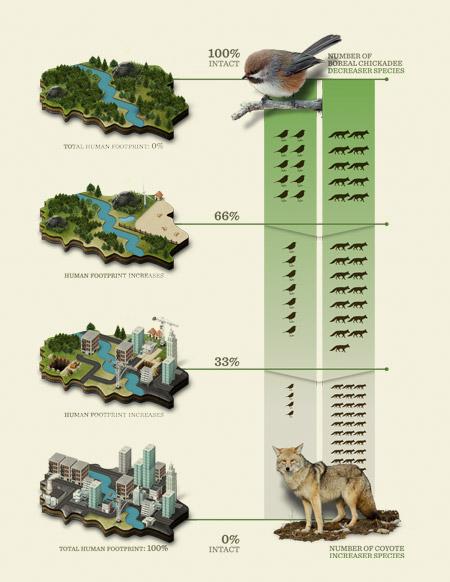
We use “arrow diagrams” to show the effects of each type of land base change on species, as well as habitat elements. To interpret the arrow diagrams, follow the arrows from the top of the figure, starting at 0% change, to the bottom to see the predicted effects on the species of:
- new forestry, then
- the effect of old regenerating harvest areas, then
- new non-forestry human footprint, then
- changes or disappearance of old non-forestry human footprint, then
- fires, and finally
- aging of undisturbed native forest.
The endpoint is the net change predicted in that species from 2010 to 2021.
Roll-up of Land Base Change Effects
For each taxonomic group we present figures which compare the effects of:
- Forestry: New forestry footprint (harvested between 2010 and 2021), regenerating old forestry footprint (harvested before 2010 and continuing to regenerate), and combined forestry effect.
- Other human footprint: New non-forestry footprint (created between 2010 and 2021), old (present before 2010), and net effect of non-forestry footprint.
- All human footprint combined.
- Natural processes: Fire (areas burned between 2010 and 2021), aging of undisturbed stands, and net change from these natural processes.
- All land base changes combined.
- 2023 Fire: areas burned in 2023.
We highlight the effects of each type of land base change on species habitat in the Southern Operating Area.
See Section 3.3 for species habitat change results.
- These changes reflect the predicted changes in species due to changes in the land base that we can map. Many other factors can also change species’ populations. We will be able to look into those when we have direct trend information, which we can then compare to the changes predicted from land base change.
- These predicted effects of land base change are based on the period 2010–2021. Harvest rates, and particularly fires, vary over time. The ABMI will soon have province-wide mapping for the year 2000, so that we can extend the attribution analysis over a longer time period.
- The results are based on ABMI habitat models, which are imperfect and improve over time as we collect more data.
Species of Conservation Concern
Species of Conservation Concern
Species of conservation concern are defined here as species that meet at least one of the following criteria:
- federally listed as Endangered, Threatened or Special Concern under Canada’s Species at Risk Act (SARA);
- provincially listed as Endangered or Threatened under Alberta’s Wildlife Act;
- recommended for listing federally by the Committee on the Status of Endangered Wildlife in Canada (COSEWIC), or provincially by Alberta’s Endangered Species Conservation Committee (ESCC) as Endangered, Threatened, or Special Concern;
- ranked as At Risk, May Be At Risk, or Sensitive in the Alberta Wild Species General Status Listing;
- ranked as S1 or S2 by the Alberta Conservation Information System (ACIMS).
See Section 4.4 for information on species of conservation concern in the Southern Operating Area, including status ranks, occurrence information, and biodiversity intactness scores for those species with enough detections.
Note that intactness is a measure of the predicted effects of local human footprint on habitat suitability; it is not a measure of population trend. Further, the ABMI cannot assess the status of all species of conservation concern in Tolko’s Southern Operating Area for one of two reasons. First, by virtue of their rarity, some species of conservation concern were simply not detected or were not detected with enough frequency to adequately assess their status. Second, the ABMI monitoring protocols are not designed to monitor some species groups, such as owls, waterfowl, and bats, that include some species of conservation concern.
Data were collected from 2003 through 2019 for birds and mosses; 2015 through 2021 for mammals; and 2003 through 2021 for lichens and vascular plants.
References
Alberta Biodiversity Monitoring Institute. 2014. Terrestrial field data collection protocols (abridged version) 2018-05-07. Alberta Biodiversity Monitoring Institute, Alberta, Canada. Report available at: abmi.ca.
Huggard, D. and L. Kremsater. 2015. Human footprint recovery for the Biodiversity Monitoring Framework—quantitative synthesis. Unpublished report.
Huggard, D. and L. Kremsater. 2015. Recommendations for forest interior and old-forest indicators for the Biodiversity Management Framework. Unpublished report.
Sólymos, P., E.T. Azeria, D.J. Huggard, M-C. Roy, and J. Schieck. 2019. Chapter 4. Predicting species status and relationships. In ABMI 10-year Science and Program Review. Report available at: https://abmi10years.ca/10-year-review/resources/
Azeria, E.R., P. Sólymos, D.J. Huggard, M-C. Roy, and J. Schieck. 2019. Detail methods and results for predicting species status and relationships. Technical Report available at: https://abmi10years.ca/10-year-review/resources/
Sólymos, P. and J. Schieck. 2016. Effects of industrial sectors on species abundance in Alberta. ABMI Science Letters, Issue 5: October, 2016.
